4. Pedigree Analysis and Population Genetics

This vignette summarizes a practical workflow for pedigree analysis with visPedigree, with emphasis on the interpretation of the main indicators used in breeding and conservation genetics.

The discussion is organized around five questions:

1. How complete and deep is the pedigree?
2. How long is the generation cycle?
3. Has genetic diversity been eroded by unequal founder use, bottlenecks, or drift?
4. How large is the effective population size under different definitions?
5. Are relationship, inbreeding, subpopulation structure, and gene flow under control?

1. Setup and Data Preparation

Different package datasets are used for different analytical tasks.

• deep_ped is useful for pedigree depth and diversity summaries.
• big_family_size_ped contains a Year column and is suitable for generation intervals.
• small_ped is convenient for relationship examples.
• inbred_ped is convenient for inbreeding and classification examples.

library(visPedigree)
library(data.table)

data(deep_ped, package = "visPedigree")
data(big_family_size_ped, package = "visPedigree")
data(small_ped, package = "visPedigree")
data(inbred_ped, package = "visPedigree")

tp_deep <- tidyped(deep_ped)
tp_small <- tidyped(small_ped)
tp_inbred <- tidyped(inbred_ped)

2. Pedigree Overview with pedstats()

pedstats() provides a compact structural summary with three components:

• $summary: pedigree size and parental structure.
• $ecg: pedigree completeness and ancestral depth.
• $gen_intervals: generation intervals, only when a usable time column is available.

Here deep_ped has no explicit birth-date column. Accordingly, pedstats() returns $summary and $ecg, whereas $gen_intervals remains NULL.

stats_deep <- pedstats(tp_deep)

stats_deep$summary
#>        N NSire  NDam NFounder MaxGen
#>    <int> <int> <int>    <int>  <int>
#> 1:  4399   483   554      138     13
tail(stats_deep$ecg)
#>         Ind      ECG FullGen MaxGen
#>      <char>    <num>   <num>  <num>
#> 1: K110997Q 7.616211       5     12
#> 2: K110997Z 6.722656       5     12
#> 3: K110998Q 4.606445       2     12
#> 4: K110998Z 6.417969       5     12
#> 5: K110999Q 7.345215       5     12
#> 6: K110999Z 6.875977       5     12
stats_deep$gen_intervals
#> NULL

# Visualize ancestral depth (Equivalent Complete Generations)
plot(stats_deep, type = "ecg", metric = "ECG")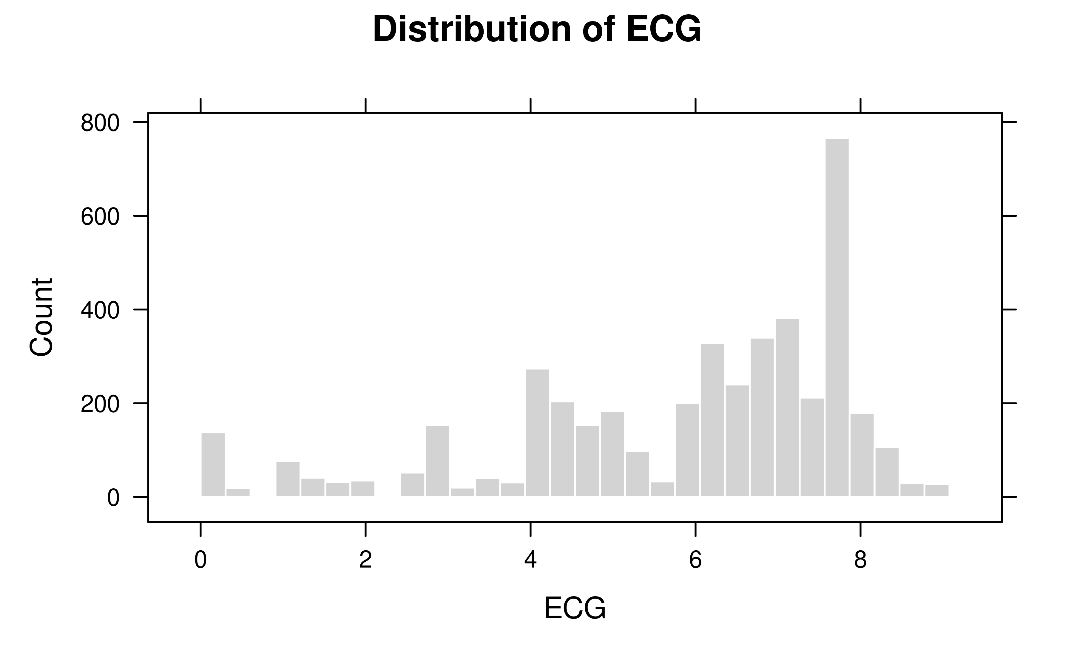

Pedigree depth and pedigree time are related but distinct quantities. The former is addressed by pedecg(), whereas the latter is addressed by pedgenint().

3. Pedigree Completeness with pedecg()

Equivalent complete generations (ECG) summarize the amount of ancestral information available for each individual:

$$ECG_i = \sum_j \left(\frac{1}{2}\right)^{g_{ij}}$$

where $g_{ij}$ is the number of generations between individual $i$ and ancestor $j$. ECG increases with both pedigree depth and pedigree completeness.

In practice:

• ECG combines depth and completeness.
• FullGen counts how many fully known ancestral generations exist.
• MaxGen records the deepest known ancestral path.

ECG is especially useful because it provides the depth adjustment required by realized effective population size estimators based on inbreeding or coancestry.

ecg_deep <- pedecg(tp_deep)

ecg_deep[order(-ECG)][1:10]
#>          Ind      ECG FullGen MaxGen
#>       <char>    <num>   <num>  <num>
#>  1: K110034Q 9.078125       6     12
#>  2: K110052L 9.078125       6     12
#>  3: K110060H 9.078125       6     12
#>  4: K110069Z 9.078125       6     12
#>  5: K110097Q 9.078125       6     12
#>  6: K110118M 9.078125       6     12
#>  7: K110131M 9.078125       6     12
#>  8: K110138M 9.078125       6     12
#>  9: K110155M 9.078125       6     12
#> 10: K110165M 9.078125       6     12

4. Generation Intervals with pedgenint()

Generation interval is the age of a parent at the birth of its offspring:

$$L = t_{offspring} - t_{parent}$$

pedgenint() estimates this quantity for seven pathway summaries:

• SS, SD, DS, DD: sex-specific gametic pathways.
• SO, DO: sex-independent sire-offspring and dam-offspring pathways.
• Average: all parent-offspring pairs combined.

The function accepts Date/POSIXct columns, date strings, or numeric years. When only an integer year is available, it is converted internally to YYYY-07-01 as a mid-year approximation.

tp_time <- tidyped(big_family_size_ped)

genint_year <- pedgenint(tp_time, timevar = "Year", unit = "year")
#> Numeric time column detected. Converting to Date (YYYY-07-01). For finer precision, convert to Date beforehand.
genint_year
#>    Pathway      N     Mean         SD
#>     <char>  <int>    <num>      <num>
#> 1: Average 280512 1.001093 0.03770707
#> 2:      DD    607 1.164398 0.37080261
#> 3:      DO 140256 1.001093 0.03770714
#> 4:      DS    507 1.196959 0.39776787
#> 5:      SD    607 1.164398 0.37080261
#> 6:      SO 140256 1.001093 0.03770714
#> 7:      SS    507 1.196959 0.39776787

# Visualize generation intervals
# Note: we can also use stats <- pedstats(tp_time, timevar = "Year") followed by plot(stats)
plot(genint_year)

The optional cycle parameter adds GenEquiv, which compares the observed mean interval with a target breeding cycle:

$$GenEquiv_i = \frac{\bar{L}_i}{L_{cycle}}$$

Values larger than 1 indicate that the realized generation interval exceeds the target cycle.

genint_cycle <- pedgenint(tp_time, timevar = "Year", unit = "year", cycle = 1.2)
#> Numeric time column detected. Converting to Date (YYYY-07-01). For finer precision, convert to Date beforehand.

genint_cycle[Pathway %in% c("SS", "SD", "DS", "DD", "Average")]
#>    Pathway      N     Mean         SD  GenEquiv
#>     <char>  <int>    <num>      <num>     <num>
#> 1: Average 280512 1.001093 0.03770707 0.8342445
#> 2:      DD    607 1.164398 0.37080261 0.9703321
#> 3:      DS    507 1.196959 0.39776787 0.9974660
#> 4:      SD    607 1.164398 0.37080261 0.9703321
#> 5:      SS    507 1.196959 0.39776787 0.9974660

5. Subpopulation Structure with pedsubpop()

Before interpreting diversity or relationship metrics, it is useful to check whether the pedigree forms a single connected population or a mixture of separate components.

pedsubpop() has two modes:

• by = NULL: summarize disconnected pedigree components.
• by = "...": summarize the pedigree by an existing grouping variable.

ped_demo <- data.table(
  Ind = c("A", "B", "C", "D", "E", "F", "G", "H"),
  Sire = c(NA, NA, "A", NA, NA, "E", NA, NA),
  Dam  = c(NA, NA, "B", NA, NA, NA, NA, NA),
  Sex = c("male", "female", "male", "female", "male", "female", "male", "female"),
  Batch = c("L1", "L1", "L1", "L1", "L2", "L2", "L3", "L3")
)

tp_demo <- tidyped(ped_demo)

pedsubpop(tp_demo)
#>       Group     N N_Sire N_Dam N_Founder
#>      <char> <int>  <num> <num>     <int>
#> 1:      GP1     3      1     1         2
#> 2:      GP2     2      1     0         1
#> 3: Isolated     3      0     0         3
pedsubpop(tp_demo, by = "Batch")
#>     Group     N N_Sire N_Dam N_Founder
#>    <char> <int>  <int> <int>     <int>
#> 1:     L1     4      1     1         3
#> 2:     L3     2      0     0         2
#> 3:     L2     2      1     0         1

This is a compact summary tool. When the actual split pedigree objects are needed for downstream analysis, use splitped().

6. Diversity Indicators with pediv()

pediv() is the integrated diversity summary. It combines:

• founder and ancestor contributions (fe, fa),
• founder genome equivalents (fg),
• retained genetic diversity (GeneDiv),
• three effective population size estimates (Ne).

All of these quantities depend on the definition of the reference population. In the present example, the reference population is defined as the most recent two generations in deep_ped.

ref_pop <- tp_deep[Gen >= max(Gen) - 1, Ind]
length(ref_pop)
#> [1] 3471

div_res <- pediv(tp_deep, reference = ref_pop, top = 10, seed = 42L)
#> Calculating founder and ancestor contributions...
#> Calculating founder contributions...
#> Calculating ancestor contributions (Boichard's iterative algorithm)...
#> Calculating Ne (coancestry) and fg...
#> Calculating Ne (inbreeding)...
#> Calculating Ne (demographic)...

div_res$summary
#>     NRef NFounder     feH       fe NAncestor     faH       fa     fafe       fg
#>    <int>    <int>   <num>    <num>     <int>   <num>    <num>    <num>    <num>
#> 1:  3471      157 92.0943 64.73344        94 60.1444 44.12033 0.681569 19.17965
#>     MeanCoan   GeneDiv NSampledCoan NeCoancestry NeInbreeding NeDemographic
#>        <num>     <num>        <int>        <num>        <num>         <num>
#> 1: 0.0260693 0.9739307         1000     124.5124     98.00425      374.2021
div_res$ancestors
#>          Ind    Contrib CumContrib  Rank
#>       <char>      <num>      <num> <int>
#>  1: K500I804 0.05248848 0.05248848     1
#>  2: K60GXQ91 0.04525893 0.09774741     2
#>  3: K60NXQ91 0.04525893 0.14300634     3
#>  4: K600532I 0.04445765 0.18746399     4
#>  5: K700S069 0.03927182 0.22673581     5
#>  6: K900D251 0.03622875 0.26296456     6
#>  7: K700S011 0.02906223 0.29202679     7
#>  8: K700U416 0.02890017 0.32092697     8
#>  9: K700U650 0.02890017 0.34982714     9
#> 10: K500I869 0.02831497 0.37814211    10

6.1 fe, fa, and fg: what do they measure?

These three indicators describe diversity loss from complementary angles.

Effective number of founders (fe)

$$f_e = \frac{1}{\sum_{i=1}^{f} p_i^2}$$

where $p_i$ is the expected contribution of founder $i$ to the reference population. fe answers the question: if all founders had contributed equally, how many founders would generate the same diversity?

Use fe when the main concern is unequal founder representation.

Effective number of ancestors (fa)

$$f_a = \frac{1}{\sum_{j=1}^{a} q_j^2}$$

where $q_j$ is the marginal contribution of ancestor $j$ after removing the contributions already explained by more influential ancestors. fa is usually smaller than fe when bottlenecks occurred.

Use fa when the main concern is genetic bottlenecks caused by a limited set of influential ancestors.

Founder genome equivalents (fg)

In its simplest interpretation,

$$f_g = \frac{1}{2\bar{C}}$$

where $\bar{C}$ is the mean coancestry of the reference population. In visPedigree, fg is estimated from a diagonal-corrected mean coancestry:

$$\hat{\bar{C}} = \frac{N-1}{N}\cdot\frac{\bar{a}_{off}}{2} + \frac{1 + \bar{F}}{2N}$$

$$f_g = \frac{1}{2\hat{\bar{C}}}$$

where $N$ is the size of the full reference population, $\bar{a}_{off}$ is the mean off-diagonal additive relationship among sampled individuals, and $\bar{F}$ is their mean inbreeding coefficient.

Use fg when the main concern is the amount of founder genome still surviving after unequal use, bottlenecks, and drift. In practice, fg is often the most conservative diversity indicator.

Retained genetic diversity (GeneDiv)

GeneDiv is the pedigree-based retained genetic diversity of the reference population:

$$GeneDiv = 1 - \bar{C}$$

where $\bar{C}$ is the same diagonal-corrected mean coancestry used to compute $f_g$. Because coancestry increases as individuals become more related by descent, $GeneDiv$ decreases towards 0 as the population becomes more uniform. An unrelated, non-inbred population has $GeneDiv = 1$; a population of full sibs from two unrelated founders has $GeneDiv \approx 0.75$.

GeneDiv and fg are both derived from $\bar{C}$, but they answer different questions. fg is measured in “equivalent number of founders” and is most useful for between-programme comparisons. GeneDiv is a dimensionless proportion and is easiest to communicate to managers and stakeholders who need a single intuitive index of diversity retention.

# GeneDiv is in the summary alongside MeanCoan
div_res$summary[, .(fg, MeanCoan, GeneDiv)]
#>          fg  MeanCoan   GeneDiv
#>       <num>     <num>     <num>
#> 1: 19.17965 0.0260693 0.9739307

6.2 Shannon-entropy effective numbers: feH and faH

The classical fe and fa are based on $\sum p_i^2$ (Hill number order $q = 2$), which is disproportionately influenced by a few large contributions. visPedigree also reports the information-theoretic counterpart at order $q = 1$, derived from Shannon entropy:

$$ f_e^{(H)} = \exp\!\Bigl(-\sum_{i=1}^{f} p_i \ln p_i\Bigr), \qquad f_a^{(H)} = \exp\!\Bigl(-\sum_{j=1}^{a} q_j \ln q_j\Bigr) $$

All four metrics satisfy a strict monotone ordering:

$$N_f \ge f_e^{(H)} \ge f_e, \qquad K \ge f_a^{(H)} \ge f_a$$

where $N_f$ is the total number of founders and $K$ is the number of ancestors considered.

Metric guide

Metric	Order	Sensitivity	What it measures
fe	$q = 2$	Dominated by common founders	Effective number of founders if contributions were equalized. Dominated by the largest contributions; many rare founders with small $p_i$ have negligible influence on the metric.
feH	$q = 1$	Balanced; sensitive to rare founders	Shannon-entropy effective founders. Counts rare founders more equitably than $q = 2$; always $\ge$fe.
fa	$q = 2$	Dominated by common ancestors	Effective number of ancestors accounting for bottleneck structure. Typically lower than fe.
faH	$q = 1$	Balanced; sensitive to rare ancestors	Shannon-entropy effective ancestors. Less dominated by the single most influential ancestor.
fg	—	Realized coancestry	Founder genome equivalents; the most conservative indicator because it captures drift as well.
GeneDiv	—	Retained diversity	Pedigree-based retained genetic diversity: $1 - \bar{C}$. Values on the $[0, 1]$ scale; higher values indicate more diversity retained relative to the base population.

Interpreting the ratio $f_e^{(H)} / f_e$

The ratio $\rho = f_e^{(H)} / f_e$ is a long-tail signal:

• $\rho \approx 1$: founder contributions are already concentrated in a small number of individuals; there is no meaningful “hidden” diversity from minor founders.
• $\rho \gg 1$: many minor founders still carry genetic material into the reference population but are effectively invisible to the classical $f_e$ metric because their contributions are small. This situation is common early in a breeding programme when the pedigree is still shallow.

The analogous ratio $f_a^{(H)} / f_a$ diagnoses the same effect at the ancestor level: a large ratio means that the bottleneck signal from the dominant ancestor is masking genuine contributions from many secondary ancestors.

Management implications

Use the two ratios together to set priorities:

1. If $f_e^{(H)} / f_e$ is large but $f_e$ itself is already high, the programme has good founder coverage; no immediate action needed.
2. If $f_e^{(H)} / f_e$ is large and $f_e$ is low, minor founders carry material that could be mobilized — consider deliberately increasing their representation in the next generation.
3. If $f_a^{(H)} / f_a$ is large, secondary ancestors are still present but marginalized; diversifying sire selection could rebalance the gene pool before their lineages are lost entirely.

# Shannon metrics are included in pediv() output
div_res$summary[, .(NFounder, feH, fe, NAncestor, faH, fa)]
#>    NFounder     feH       fe NAncestor     faH       fa
#>       <int>   <num>    <num>     <int>   <num>    <num>
#> 1:      157 92.0943 64.73344        94 60.1444 44.12033

# The ratio feH/fe reveals long-tail founder diversity
div_res$summary[, .(rho_founder = feH / fe, rho_ancestor = faH / fa)]
#>    rho_founder rho_ancestor
#>          <num>        <num>
#> 1:     1.42267      1.36319

# pedcontrib() provides the same metrics via its summary
contrib_res <- pedcontrib(tp_deep, reference = ref_pop, mode = "both")
#> Calculating founder contributions...
#> Calculating ancestor contributions (Boichard's iterative algorithm)...
contrib_res$summary[c("n_founder", "f_e_H", "f_e", "n_ancestor", "f_a_H", "f_a")]
#> $n_founder
#> [1] 157
#> 
#> $f_e_H
#> [1] 92.0943
#> 
#> $f_e
#> [1] 64.73344
#> 
#> $n_ancestor
#> [1] 94
#> 
#> $f_a_H
#> [1] 60.1444
#> 
#> $f_a
#> [1] 44.12033

7. Diversity Dynamics over Time with pedhalflife()

pediv() provides a static snapshot of diversity. When multiple time points (generations, years, etc.) are available, pedhalflife() tracks how $f_e$, $f_a$, and $f_g$ evolve and fits a log-linear decay model to quantify the rate of diversity loss.

The total loss rate $\lambda_{total}$ is decomposed into three additive components that each have a distinct biological meaning:

Component	Symbol	Source of loss
Foundation	$\lambda_e$	Unequal founder contributions
Bottleneck	$\lambda_b$	Overuse of key ancestors
Drift	$\lambda_d$	Random sampling loss

The diversity half-life is the number of time units for $f_g$ to halve: $$T_{1/2} = \frac{\ln 2}{\lambda_{total}}$$

hl <- pedhalflife(tp_deep, timevar = "Gen")
#> Calculating diversity across 13 time points...
print(hl)
#> Information-Theoretic Diversity Half-Life
#> -----------------------------------------
#> Total Loss Rate (lambda_total):   0.128778
#>   Foundation  (lambda_e)      :   0.034626
#>   Bottleneck  (lambda_b)      :   0.025217
#>   Drift       (lambda_d)      :   0.068935
#> -----------------------------------------
#> Diversity Half-life (T_1/2)   :       5.38 (Gen)
#> 
#> Timeseries: 13 time points

The printed half-life shows the unit in parentheses — (Gen) here — taken directly from the timevar argument. The full object exposes three components:

• hl$timeseries — per-time-point table (see column guide below).
• hl$decay — single-row table with LambdaE, LambdaB, LambdaD, LambdaTotal, and THalf.
• hl$timevar — the timevar string passed to the call.

7.1 Column guide for $timeseries

The cascade rests on a simple algebraic identity:

$$\ln f_g = \underbrace{\ln f_e}_{\texttt{lnfe}} + \underbrace{\ln\!\left(\frac{f_a}{f_e}\right)}_{\texttt{lnfafe}} + \underbrace{\ln\!\left(\frac{f_g}{f_a}\right)}_{\texttt{lnfgfa}}$$

Because OLS is linear, the slope of $\ln f_g$ versus time equals the sum of the slopes of the three right-hand terms. This guarantees exact additivity: $\lambda_{total} = \lambda_e + \lambda_b + \lambda_d$.

Column	Formula	What it measures
lnfe	$\ln f_e$	Log effective-founder diversity. Declines when founder contributions become more unequal over time.
lnfa	$\ln f_a$	Log effective-ancestor diversity. Lies below lnfe whenever bottleneck ancestors have been over-used.
lnfg	$\ln f_g$	Log founder-genome equivalents. The most comprehensive diversity signal; integrates founder use, bottlenecks, and drift.
lnfafe	$\ln(f_a/f_e)$	Bottleneck gap. When this ratio decreases over time, a small number of ancestors dominate the gene pool even beyond what unequal founder use would predict.
lnfgfa	$\ln(f_g/f_a)$	Drift gap. Captures random allele loss due to finite population size. Because $f_g \le f_a$ always, this term is $\le 0$ and becomes more negative as genetic drift accumulates.
TimeStep	numeric	OLS time axis (same as Time for numeric timevar; sequential indices otherwise).

7.2 Interpreting the $\lambda$ components

The negative OLS slope of each log column gives the corresponding loss rate. All three terms have a distinct policy implication:

$\lambda_e$ (Foundation) — rate of increase in founder-contribution inequality. A large $\lambda_e$ suggests that founder representation is still diverging, possibly because some founders are reaching later generations through many more breeding pathways than others. Remedy: broaden founder use in the breeding programme.

$\lambda_b$ (Bottleneck) — rate at which a few key ancestors capture an ever-larger share of the gene pool beyond what founder inequality alone explains. A large $\lambda_b$ points to systematic over-selection of certain families or sires. Remedy: restrict the number of offspring per high-ranking animal; rotate breeding males.

$\lambda_d$ (Drift) — rate of random allele loss in finite populations. This component is always present and increases with small effective population size. It is the only component that cannot be reversed by changing selection decisions; it can only be slowed by maintaining a larger breeding population or by cryopreservation of genetic material.

When $\lambda_d \gg \lambda_e + \lambda_b$ (as in the example above), drift is the dominant driver of diversity loss and should be the primary management target.

7.3 Interpreting $T_{1/2}$

$T_{1/2}$ is the number of time units (generations, years, etc.) required for $f_g$ to fall to half its current value, assuming the observed decay rate continues. It is a single headline figure that combines all three loss channels.

As a rough benchmark: a half-life shorter than five to ten generations is generally considered a cause for concern in conservation and aquaculture genetics. Breed registries and conservation programmes often use $T_{1/2}$ as a threshold indicator for triggering corrective management.

hl$timeseries
#>      Time  NRef        fe        fa         fg     lnfe     lnfa     lnfg
#>     <int> <int>     <num>     <num>      <num>    <num>    <num>    <num>
#>  1:     1   138 138.00000 138.00000 138.000000 4.927254 4.927254 4.927254
#>  2:     2    96  81.55752  74.02410  57.242236 4.401309 4.304391 4.047292
#>  3:     3    74  69.53651  55.45316  36.204959 4.241852 4.015539 3.589196
#>  4:     4    91  33.07439  22.47218  18.505028 3.498759 3.112278 2.918042
#>  5:     5    95  58.21114  26.60280  17.148880 4.064077 3.281016 2.841933
#>  6:     6   119  20.87729  13.46723   9.709381 3.038662 2.600259 2.273093
#>  7:     7    37  40.12238  24.89445  10.016763 3.691934 3.214645 2.304260
#>  8:     8    41  43.07344  23.20121   9.927020 3.762907 3.144204 2.295260
#>  9:     9    51  43.45747  25.55284  11.468733 3.771783 3.240749 2.439624
#> 10:    10    78  58.80040  35.70455  14.967166 4.074149 3.575278 2.705859
#> 11:    11   108  49.32442  33.37264  14.920611 3.898419 3.507737 2.702744
#> 12:    12   209  51.27256  33.93121  14.728712 3.937156 3.524335 2.689799
#> 13:    13  3262  65.47682  44.33880  19.682156 4.181696 3.791860 2.979712
#>         lnfafe     lnfgfa TimeStep
#>          <num>      <num>    <num>
#>  1:  0.0000000  0.0000000        1
#>  2: -0.0969179 -0.2570986        2
#>  3: -0.2263131 -0.4263427        3
#>  4: -0.3864809 -0.1942358        4
#>  5: -0.7830602 -0.4390836        5
#>  6: -0.4384028 -0.3271666        6
#>  7: -0.4772897 -0.9103847        7
#>  8: -0.6187023 -0.8489440        8
#>  9: -0.5310341 -0.8011241        9
#> 10: -0.4988704 -0.8694193       10
#> 11: -0.3906828 -0.8049930       11
#> 12: -0.4128205 -0.8345365       12
#> 13: -0.3898361 -0.8121477       13

To focus on a specific time window, pass the desired values to the at argument:

hl_recent <- pedhalflife(tp_deep, timevar = "Gen",
                         at = tail(sort(unique(tp_deep$Gen)), 4))
#> Calculating diversity across 4 time points...
print(hl_recent)
#> Information-Theoretic Diversity Half-Life
#> -----------------------------------------
#> Total Loss Rate (lambda_total):  -0.077122
#>   Foundation  (lambda_e)      :  -0.036138
#>   Bottleneck  (lambda_b)      :  -0.030497
#>   Drift       (lambda_d)      :  -0.010487
#> -----------------------------------------
#> Diversity Half-life (T_1/2)   : NA
#> 
#> Timeseries: 4 time points

Plotting the object shows the log-linear decay of each diversity metric:

plot(hl, type = "log")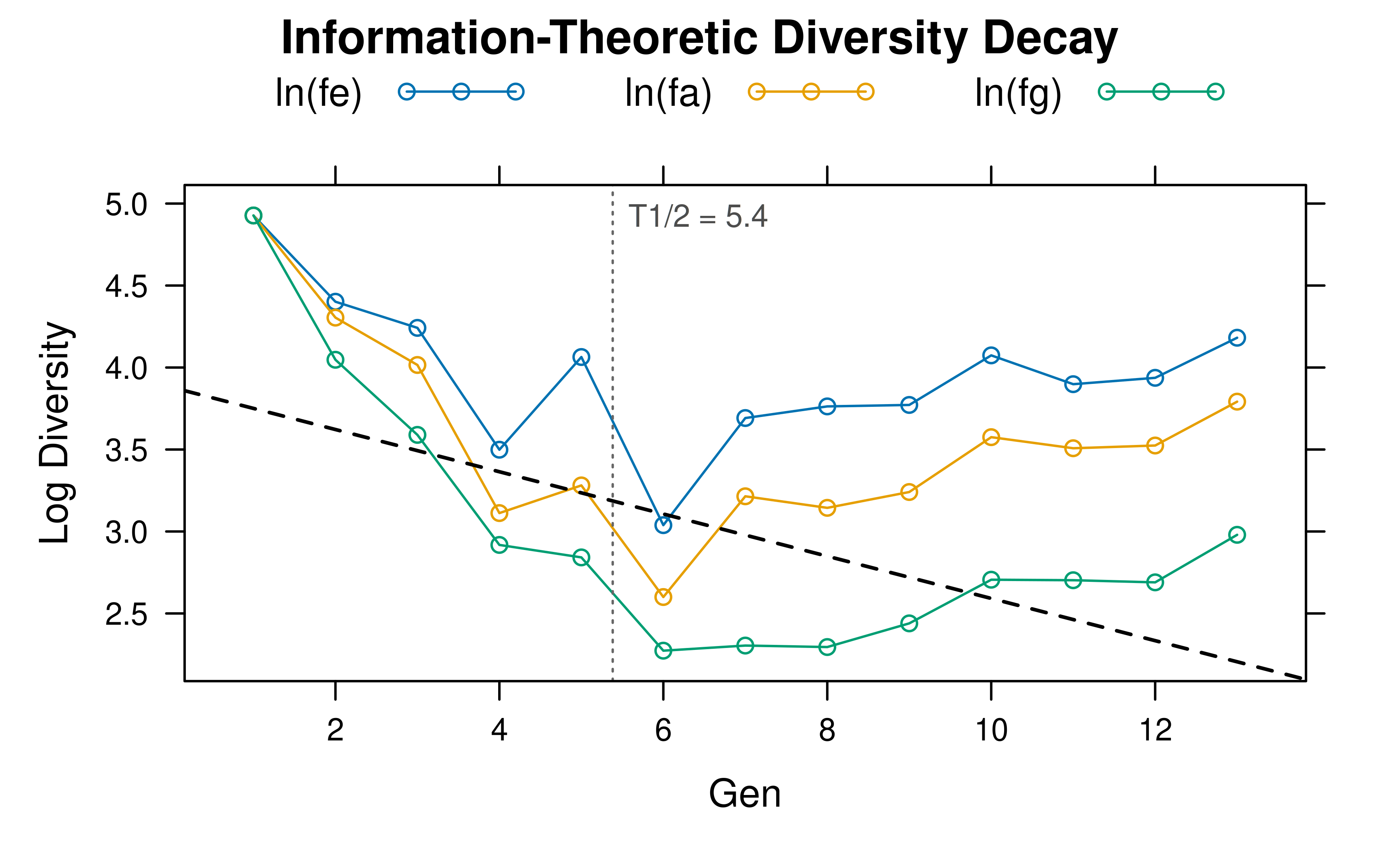

A type = "raw" plot shows the equivalent numbers on the original scale:

plot(hl, type = "raw")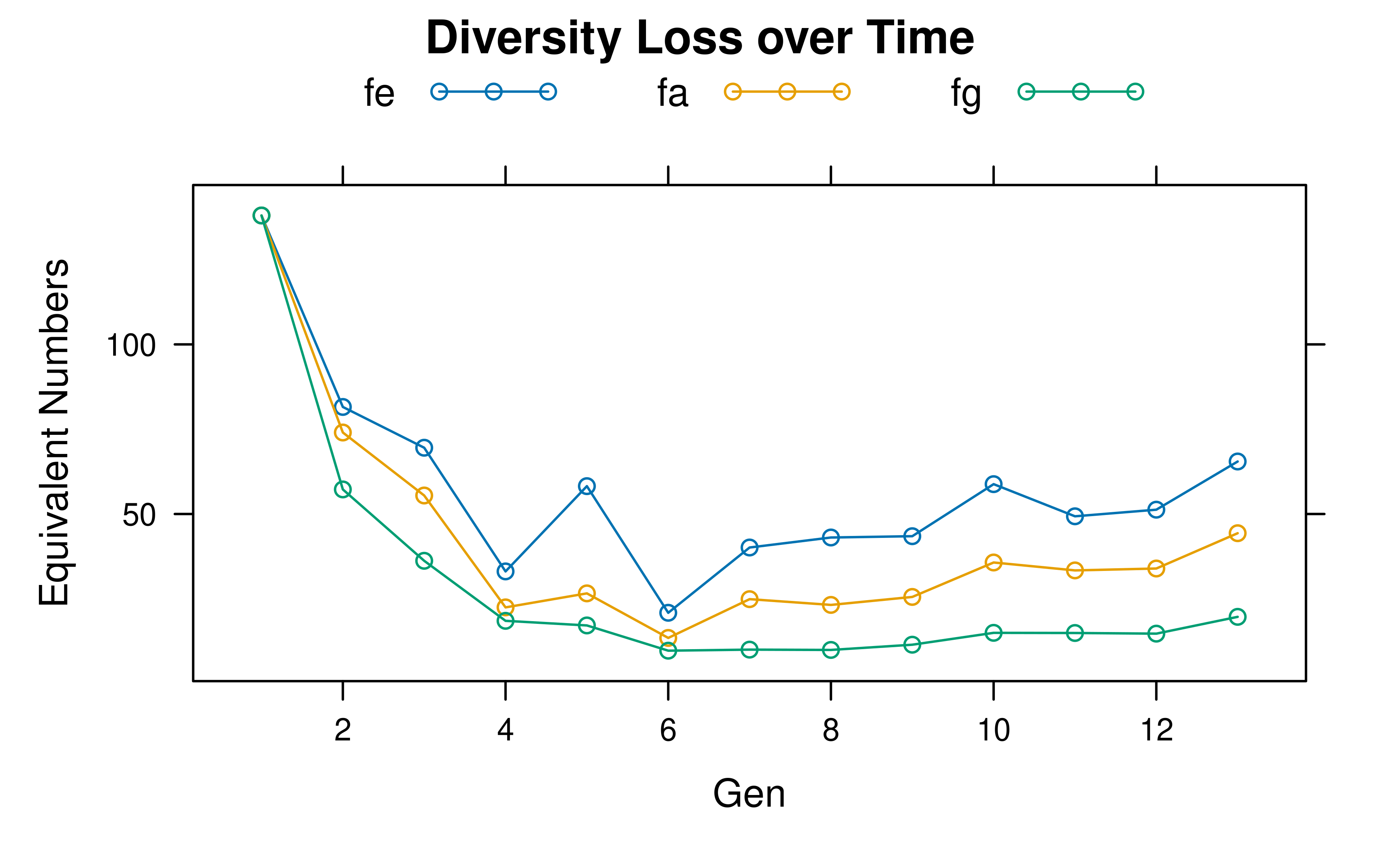

8. Effective Population Size with pedne() and pediv()

pediv() reports three complementary effective population size definitions. Each addresses a distinct biological question.

8.1 Demographic Ne

$$N_e = \frac{4 N_m N_f}{N_m + N_f}$$

where $N_m$ and $N_f$ are the numbers of contributing males and females. This is the easiest estimate to understand, but it ignores realized pedigree structure, inbreeding, and drift. It is therefore often optimistic.

8.2 Inbreeding Ne

$$\Delta F_i = 1 - (1 - F_i)^{1/(ECG_i - 1)}$$

$$N_e = \frac{1}{2\overline{\Delta F}}$$

This estimator uses the realized rate of inbreeding. ECG standardizes individuals with different pedigree depths. Use this estimate when the primary concern is the rate of inbreeding accumulation.

8.3 Coancestry Ne

$$\Delta c_{ij} = 1 - (1 - c_{ij})^{1/(\frac{ECG_i + ECG_j}{2})}$$

$$N_e = \frac{1}{2\overline{\Delta c}}$$

This estimator is based on the rate of coancestry among members of the reference population. Because it captures the accumulation of relatedness before it is fully expressed as realized inbreeding, it is often the strictest and most sensitive warning signal in managed breeding populations.

9. Average Relationship Trends with pedrel()

pedrel() summarizes pairwise relatedness within groups. Two complementary scales are available via the scale argument.

9.1 Mean additive relationship (scale = "relationship")

The default scale returns the mean off-diagonal additive relationship:

$$MeanRel = \frac{1}{n(n-1)} \sum_{i \ne j} a_{ij}$$

where $a_{ij} = 2c_{ij}$ is the additive relationship and $c_{ij}$ is the coancestry (kinship coefficient) between individuals $i$ and $j$. A higher MeanRel means that individuals within the group are, on average, more related by descent.

tp_small$BirthYear <- 2010 + tp_small$Gen

rel_by_gen <- pedrel(tp_small, by = "Gen")
rel_by_gen
#>      Gen NTotal NUsed   MeanRel
#>    <int>  <int> <int>     <num>
#> 1:     1      9     9 0.0000000
#> 2:     2      5     5 0.2000000
#> 3:     3      7     7 0.1547619
#> 4:     4      3     3 0.1145833
#> 5:     5      2     2 0.0468750
#> 6:     6      2     2 0.5507812

The reference argument lets you focus on a subset of interest inside each group, such as candidate breeders.

ref_ids <- c("Z1", "Z2", "X", "Y")

pedrel(tp_small, by = "Gen", reference = ref_ids)
#> Warning in FUN(X[[i]], ...): Group '1' has less than 2 individuals after
#> applying 'reference', returning NA_real_.
#> Warning in FUN(X[[i]], ...): Group '2' has less than 2 individuals after
#> applying 'reference', returning NA_real_.
#> Warning in FUN(X[[i]], ...): Group '3' has less than 2 individuals after
#> applying 'reference', returning NA_real_.
#> Warning in FUN(X[[i]], ...): Group '4' has less than 2 individuals after
#> applying 'reference', returning NA_real_.
#>      Gen NTotal NUsed   MeanRel
#>    <int>  <int> <int>     <num>
#> 1:     1      9     0        NA
#> 2:     2      5     0        NA
#> 3:     3      7     0        NA
#> 4:     4      3     0        NA
#> 5:     5      2     2 0.0468750
#> 6:     6      2     2 0.5507812

9.2 Corrected mean coancestry (scale = "coancestry")

When scale = "coancestry", pedrel() returns the diagonal-corrected population mean coancestry following Caballero & Toro (2000):

$$\bar{C} = \frac{N - 1}{N} \cdot \frac{\bar{a}_{off}}{2} + \frac{1 + \bar{F}}{2N}$$

where $\bar{a}_{off}$ is the mean off-diagonal relationship, $\bar{F}$ is the mean inbreeding coefficient of the group, and $N$ is the group size. This $\bar{C}$ accounts for self-coancestry within the group and matches the internal coancestry quantity used by pediv() to derive $f_g$.

coan_by_gen <- pedrel(tp_small, by = "Gen", scale = "coancestry")
coan_by_gen
#>      Gen NTotal NUsed   MeanCoan
#>    <int>  <int> <int>      <num>
#> 1:     1      9     9 0.05555556
#> 2:     2      5     5 0.18000000
#> 3:     3      7     7 0.13775510
#> 4:     4      3     3 0.20833333
#> 5:     5      2     2 0.27148438
#> 6:     6      2     2 0.39550781

Use scale = "relationship" to track mean pairwise relatedness trends. Use scale = "coancestry" when you need a population-level coancestry consistent with diversity metrics from pediv().

pedrel(scale = "coancestry") applies the same diagonal-corrected formula as pediv(). The resulting MeanCoan values are therefore directly comparable to pediv()$summary$MeanCoan, and GeneDiv = 1 - MeanCoan translates the trend table from pedrel() into a retained-diversity timeline without any additional computation.

MeanRel and coancestry-based Ne are conceptually linked, but they are not identical summaries. MeanRel is an average additive relationship within a group, whereas coancestry-based Ne is derived from the rate of increase in coancestry across pedigree depth.

10. Inbreeding Trends with inbreed() and pedfclass()

Wright’s inbreeding coefficient $F$ is the probability that the two alleles of an individual are identical by descent. A practical starting point is to inspect the mean trend by generation.

tp_inbred_f <- inbreed(tp_inbred)

f_trend <- tp_inbred_f[, .(MeanF = mean(f, na.rm = TRUE)), by = Gen]
f_trend
#>      Gen  MeanF
#>    <int>  <num>
#> 1:     1 0.0000
#> 2:     2 0.0000
#> 3:     3 0.2500
#> 4:     4 0.2500
#> 5:     5 0.4375

For classification by inbreeding severity, pedfclass() can be applied directly to the pedigree object. If the inbreeding coefficient is not yet present, the function computes it internally.

pedfclass(tp_inbred)
#> Calculating inbreeding coefficients...
#> Key: <FClass>
#>                 FClass Count Percentage
#>                  <ord> <int>      <num>
#> 1:               F = 0     4   57.14286
#> 2:     0 < F <= 0.0625     0    0.00000
#> 3: 0.0625 < F <= 0.125     0    0.00000
#> 4:   0.125 < F <= 0.25     2   28.57143
#> 5:            F > 0.25     1   14.28571

Custom reporting thresholds can be supplied through breaks.

pedfclass(tp_inbred, breaks = c(0.03125, 0.0625, 0.125, 0.25))
#> Calculating inbreeding coefficients...
#> Key: <FClass>
#>                   FClass Count Percentage
#>                    <ord> <int>      <num>
#> 1:                 F = 0     4   57.14286
#> 2:      0 < F <= 0.03125     0    0.00000
#> 3: 0.03125 < F <= 0.0625     0    0.00000
#> 4:   0.0625 < F <= 0.125     0    0.00000
#> 5:     0.125 < F <= 0.25     2   28.57143
#> 6:              F > 0.25     1   14.28571

The default thresholds correspond approximately to familiar pedigree scenarios:

• $F = 0.0625$: half-sib mating.
• $F = 0.125$: avuncular or grandparent-grandchild mating.
• $F = 0.25$: full-sib or parent-offspring mating.

11. Gene Flow and Partial Inbreeding

11.1 pedancestry(): founder-line proportions

pedancestry() tracks how founder groups contribute to later descendants. This is useful when founders are labeled by line, strain, or geographic origin.

ped_line <- data.table(
  Ind = c("A", "B", "C", "D", "E", "F", "G"),
  Sire = c(NA, NA, NA, NA, "A", "C", "E"),
  Dam  = c(NA, NA, NA, NA, "B", "D", "F"),
  Sex = c("male", "female", "male", "female", "male", "female", "male"),
  Line = c("Line1", "Line1", "Line2", "Line2", NA, NA, NA)
)

tp_line <- tidyped(ped_line)

anc <- pedancestry(tp_line, foundervar = "Line")
anc
#>       Ind Line1 Line2
#>    <char> <num> <num>
#> 1:      A   1.0   0.0
#> 2:      B   1.0   0.0
#> 3:      C   0.0   1.0
#> 4:      D   0.0   1.0
#> 5:      E   1.0   0.0
#> 6:      F   0.0   1.0
#> 7:      G   0.5   0.5

11.2 pedpartial(): which ancestors explain inbreeding?

pedpartial() decomposes total inbreeding into contributions from selected ancestors. It is useful for identifying which ancestors are most responsible for the observed inbreeding.

partial_f <- pedpartial(tp_inbred, ancestors = c("A", "B"))
#> Calculating partial inbreeding for 2 ancestors...
partial_f
#>       Ind       A       B
#>    <char>   <num>   <num>
#> 1:      A 0.00000 0.00000
#> 2:      B 0.00000 0.00000
#> 3:      C 0.00000 0.00000
#> 4:      D 0.00000 0.00000
#> 5:      E 0.12500 0.12500
#> 6:      F 0.00000 0.25000
#> 7:      G 0.15625 0.28125

12. Practical Interpretation

One useful interpretation order is:

1. Check pedigree depth and completeness with pedecg().
2. Check generation timing with pedgenint().
3. Quantify static diversity with fe, fa, fg, and GeneDiv via pediv(); compare with feH and faH to assess long-tail founder value. Use GeneDiv (= $1 - \bar{C}$) as the headline retained-diversity index for management reporting.
4. Track diversity dynamics over time with pedhalflife(). Inspect $\lambda_e$, $\lambda_b$, and $\lambda_d$ to identify the dominant driver of loss; use $T_{1/2}$ as a headline indicator for management reporting.
5. Compare demographic, inbreeding, and coancestry-based Ne.
6. Monitor MeanRel and MeanF over time.
7. Use pedsubpop(), pedancestry(), and pedpartial() to diagnose structure, introgression, and bottlenecks.

References

• Boichard, D., Maignel, L., & Verrier, É. (1997). The value of using probabilities of gene origin to measure genetic variability in a population. Genetics Selection Evolution, 29(1), 5-23.
• Caballero, A., & Toro, M. A. (2000). Interrelations between effective population size and other pedigree tools for the management of conserved populations. Genetical Research, 75(3), 331-343.
• Cervantes, I., Goyache, F., Molina, A., Valera, M., & Gutiérrez, J. P. (2011). Estimation of effective population size from the rate of coancestry in pedigreed populations. Journal of Animal Breeding and Genetics, 128(1), 56-63.
• Gutiérrez, J. P., Cervantes, I., Molina, A., Valera, M., & Goyache, F. (2008). Individual increase in inbreeding allows estimating effective sizes from pedigrees. Genetics Selection Evolution, 40(4), 359-378.
• Gutiérrez, J. P., Cervantes, I., & Goyache, F. (2009). Improving the estimation of realized effective population sizes in farm animals. Journal of Animal Breeding and Genetics, 126(4), 327-332.
• Hill, M. O. (1973). Diversity and evenness: a unifying notation and its consequences. Ecology, 54(2), 427-432.
• Jost, L. (2006). Entropy and diversity. Oikos, 113(2), 363-375.
• Lacy, R. C. (1989). Analysis of founder representation in pedigrees: founder equivalents and founder genome equivalents. Zoo Biology, 8(2), 111-123.
• Wright, S. (1922). Coefficients of inbreeding and relationship. The American Naturalist, 56(645), 330-338.
• Wright, S. (1931). Evolution in Mendelian populations. Genetics, 16(2), 97-159.