5. Calculation and visualization of relationship matrix

Calculating Relationship Matrices with pedmat()
1.1 Supported Methods
1.2 Basic Usage
1.3 Sparse Matrix Representation
Matrix-Free Products with pedprod()
2.1 When to Use pedprod vs pedmat
2.2 Basic Usage — $Ax$ (vector)
2.3 Products with $A^{-1}$
2.4 Multiple Contribution Schemes — $AX$
2.5 Practical Use Cases
2.6 Performance and Scalability
Inspecting the Matrix
3.1 Summary Statistics
3.2 Querying Specific Relationships
Compact Mode for Large Pedigrees
4.1 Using compact = TRUE
4.2 Expanding and Querying Compacted Matrices
4.3 When to Use Compact Mode
Visualizing Relationship Matrices with vismat()
5.1 Relationship Heatmaps
5.2 Inbreeding and Kinship Histograms
Performance Considerations

Relationship matrices are fundamental tools in quantitative genetics and animal breeding. They quantify the genetic similarity between individuals due to shared ancestry, which is essential for estimating breeding values (BLUP) and managing genetic diversity. The visPedigree package provides efficient tools for calculating various relationship matrices and visualizing them through heatmaps and histograms.

1. Calculating Relationship Matrices with `pedmat()`

The pedmat() function is the primary tool for calculating relationship matrices. It supports both additive and dominance relationship matrices, as well as their inverses. The inverse additive relationship matrix (Ainv) follows Henderson’s rules (Henderson, 1976), while inbreeding coefficients use the same optimized recursive engine as inbreed(), based on algorithms for large populations described by Meuwissen & Luo (1992) and Sargolzaei et al. (2005).

1.1 Supported Methods

The method parameter in pedmat() determines the type of matrix to calculate:

“A”: Additive relationship matrix (Numerator Relationship Matrix).
“Ainv”: Inverse of the additive relationship matrix.
“D”: Dominance relationship matrix.
“Dinv”: Inverse of the dominance relationship matrix.
“AA”: Additive-by-additive (epistatic) relationship matrix.
“AAinv”: Inverse of the epistatic relationship matrix.
“f”: Inbreeding coefficients vector (uses the same optimized engine as tidyped(..., inbreed = TRUE)).

1.2 Basic Usage

Most calculations require a pedigree tidied by tidyped().

# Load example pedigree and tidy it
data(small_ped)
tped <- tidyped(small_ped)

# Calculate Additive Relationship Matrix (A)
mat_A <- pedmat(tped, method = "A")

# Calculate Dominance Relationship Matrix (D)
mat_D <- pedmat(tped, method = "D")

# Calculate inbreeding coefficients (f)
vec_f <- pedmat(tped, method = "f")

1.3 Sparse Matrix Representation

By default, pedmat() returns a sparse matrix (class dsCMatrix from the Matrix package) for relationship matrices. This is highly memory-efficient for large pedigrees where many individuals are unrelated.

class(mat_A)
#> [1] "dgeMatrix"
#> attr(,"package")
#> [1] "Matrix"

2. Matrix-Free Products with `pedprod()`

For small and moderate pedigrees, matrices returned by pedmat() are ordinary matrix-like R objects and can be used directly with R’s %*%. For large pedigrees, however, forming the dense additive relationship matrix can be the dominant memory cost. pedprod() instead computes $Ax$ , $AX$ , $A^{-1}x$ , or $A^{-1}X$ directly from the pedigree — without ever constructing the $n \times n$ relationship matrix.

The implementation uses the pedigree factorization $A = TDT'$ (Colleau, 2002), where $T$ is the transmission matrix and $D$ is the diagonal matrix of Mendelian sampling variances. The product is computed through backward and forward pedigree traversals in $O(np)$ time for an $n \times p$ right-hand side, with $O(np)$ working memory — a fraction of the $O(n^2)$ storage that a dense $A$ would require.

2.1 When to Use `pedprod` vs `pedmat`

Use `pedprod()` when …	Use `pedmat()` when …
You only need matrix-vector products ( $Ax$ , $A^{-1}x$ )	You need individual relationship coefficients
The pedigree has >10 000 individuals	The pedigree is small enough that $A$ fits in memory
You are iterating (e.g., BLUP, OCS, MCMC)	You need the matrix for visualization or inspection
Memory is the bottleneck	You need $D$ , $AA$ , or dominance matrices
You are working with $A^{-1}$ products for mixed models	You need to query specific pairwise relationships

The two functions are complementary: pedmat() gives you the full matrix when you need to examine it; pedprod() applies the matrix implicitly when you only need its action on vectors.

2.2 Basic Usage — $A x$ (vector)

The most common use is computing the additive relationship of every individual to a weighted group — for example, a set of selection candidates.

# Load example pedigree and tidy it
data(small_ped)
tped <- tidyped(small_ped)

# Equal contributions from two candidates; other individuals have zero weight
weights <- c(Z1 = 0.5, Z2 = 0.5)

# Relationship of every pedigree individual to the weighted candidate group
Ax <- pedprod(tped, weights)
head(Ax)
#>       A       B       F       I      J1      J2 
#> 0.09375 0.09375 0.06250 0.00000 0.06250 0.12500

# Average additive relationship c' A c and average coancestry
mean_relationship <- sum(weights * Ax[names(weights)])
mean_coancestry <- mean_relationship / 2
c(mean_relationship = mean_relationship, mean_coancestry = mean_coancestry)
#> mean_relationship   mean_coancestry 
#>         0.7910156         0.3955078

Named vs unnamed vectors. When x is named, individuals not listed automatically receive value zero — you do not need to pad the vector yourself. An unnamed vector must have exactly one entry per pedigree individual in IndNum order:

# Named: only listed individuals get non-zero values
named_x <- c(Z1 = 0.3, Z2 = 0.4, A = 0.3)
pedprod(tped, named_x)[1:6]  # B, C, etc. are automatically zero
#>        A        B        F        I       J1       J2 
#> 0.365625 0.065625 0.043750 0.000000 0.043750 0.087500

# Unnamed: must match the pedigree size
unnamed_x <- rep(1, nrow(tped))
length(pedprod(tped, unnamed_x))
#> [1] 28

Input validation catches common mistakes: duplicate or unknown IDs, missing values, and non-finite entries are all rejected with informative messages.

2.3 Products with $A^{-1}$

The inverse additive relationship matrix $A^{-1}$ is fundamental in mixed model equations (Henderson’s BLUP). pedprod() computes $A^{-1}x$ and $A^{-1}X$ efficiently using Henderson’s rules without forming the $n \times n$ matrix:

# Ainv * vector
x <- rnorm(nrow(tped))
Ainv_x <- pedprod(tped, x, method = "Ainv")
head(Ainv_x)
#>           A           B           F           I          J1          J2 
#> -2.90971042 -1.25434985 -2.89496064 -1.67763900  0.05803645  2.47858892

# Verify against explicit computation (small pedigree only)
A <- pedmat(tped, method = "A", sparse = FALSE)
Ainv <- pedmat(tped, method = "Ainv", sparse = FALSE)
all.equal(
  unname(Ainv_x),
  unname(drop(Ainv %*% x)),
  tolerance = 1e-12
)
#> [1] TRUE

For large pedigrees where explicit inversion is impossible, pedprod(tped, x, method = "Ainv") remains computationally feasible. The numerical equivalence with the full matrix can be verified on a small pedigree:

# Ainv * (A * x) should recover x (to machine precision)
A_x <- pedprod(tped, x, method = "A")
Ainv_Ax <- pedprod(tped, A_x, method = "Ainv")
all.equal(unname(Ainv_Ax), unname(x), tolerance = 1e-12)
#> [1] TRUE

2.4 Multiple Contribution Schemes — $A X$

When x is a matrix, pedprod() computes all columns in a single backward/ forward traversal of the pedigree. This is significantly more efficient than calling pedprod() repeatedly for each column.

# Three ways to weight the SAME two candidates (Z1 and Z2 are full sibs)
schemes <- cbind(
  Equal      = c(Z1 = 0.5, Z2 = 0.5),
  Z1_only    = c(Z1 = 1.0, Z2 = 0.0),
  Weighted   = c(Z1 = 0.7, Z2 = 0.3)
)
AX <- pedprod(tped, schemes)

# The schemes diverge at the candidates themselves (and their descendants);
# a shared ancestor is equally related to any weighting of two full sibs.
AX[c("Z1", "Z2"), ]
#>        Equal   Z1_only  Weighted
#> Z1 0.7910156 1.0312500 0.8871094
#> Z2 0.7910156 0.5507812 0.6949219

# Expected average relationship within each contributing group, 0.5 * c'A c.
# Under random mating this equals the mean inbreeding of the resulting progeny.
group_coancestry <- 0.5 * colSums(schemes * AX[rownames(schemes), ])
round(group_coancestry, 5)
#>    Equal  Z1_only Weighted 
#>  0.39551  0.51562  0.41473

The three schemes draw on the same two full sibs, yet the genetic consequence differs sharply. Concentrating all contribution on a single animal (Z1_only) exposes its full, partly inbred genome and inflates the group’s expected progeny inbreeding to 0.516, whereas spreading contribution evenly (Equal) drives it down to 0.396. Trading a little short-term gain for a lower average relationship is exactly the balance struck by optimal contribution selection. pedprod() supplies the underlying $c'A c$ evaluation for every candidate column in a single $O(np)$ traversal — compared to $O(p \cdot n^2)$ for explicit products with a precomputed $A$ — and never forms $A$ itself.

2.5 Practical Use Cases

Optimal Contribution Selection (OCS)

OCS maximizes genetic gain while constraining inbreeding. The core computation repeatedly evaluates $c'A c$ for candidate contribution vectors $c$ :

# Weighted candidate contributions
candidates <- setNames(c(0.25, 0.25, 0.25, 0.25), c("Z1", "Z2", "A", "B"))
Ac <- pedprod(tped, candidates)

# Average coancestry of the selected group: 0.5 * c' A c
c_accepted <- sum(candidates * Ac[names(candidates)]) / 2
c_accepted
#> [1] 0.1848145

With pedprod(), this evaluation is fast enough to be embedded inside an iterative optimization loop over thousands of candidate configurations.

Mixed Model Equations

The mixed model equations for BLUP require products $A^{-1} u$ and $A^{-1} Z$ . For an $n \times p$ design matrix $Z$ , use:

# Simulated breeding values as a matrix right-hand side
set.seed(20260704)
Z_design <- cbind(
  trait1 = rnorm(nrow(tped)),
  trait2 = rnorm(nrow(tped))
)
rownames(Z_design) <- tped$Ind

# Ainv * Z in one traversal — no Ainv ever stored
Ainv_Z <- pedprod(tped, Z_design, method = "Ainv")
dim(Ainv_Z)
#> [1] 28  2
Ainv_Z[1:5, ]
#>       trait1     trait2
#> A  -2.731207 -1.7418085
#> B  -1.352460 -1.5616321
#> F   4.209353 -2.7144441
#> I  -1.330313  0.4133992
#> J1 -2.663064 -0.7030142

Founder Contribution Analysis

Isolating one founder at a time turns pedprod() into a founder-origin decomposition: the product $A e_f$ (a unit vector on founder $f$ ) returns that founder’s expected genetic contribution to every individual. Stacking the unit vectors into a matrix decomposes the whole population in one traversal, exposing which founders dominate the current gene pool and which have been lost:

# One unit contribution vector per founder: column f isolates founder f
founder_ids <- tped[Gen == 1, Ind]
founder_design <- diag(length(founder_ids))
dimnames(founder_design) <- list(founder_ids, founder_ids)

# A %*% e_f is founder f's expected genetic contribution to every individual
footprint <- pedprod(tped, founder_design, method = "A")

# Founder composition of one candidate: contributions sum to one
round(footprint["Z1", ], 4)
#>      A      B      F      I     J1     J2      N      O      R 
#> 0.0938 0.0938 0.0625 0.0000 0.0625 0.1250 0.5312 0.0312 0.0000

# Average founder contribution to the youngest generation, ranked
young <- tped[Gen == max(Gen), Ind]
founder_share <- sort(colMeans(footprint[young, , drop = FALSE]), decreasing = TRUE)
round(founder_share, 4)
#>      N     J2      A      B      F     J1      O      I      R 
#> 0.5312 0.1250 0.0938 0.0938 0.0625 0.0625 0.0312 0.0000 0.0000

Reading across a row (footprint["Z1", ]) decomposes an individual’s genome into founder origins that sum to one; reading down a column isolates a single founder’s footprint across the pedigree. Here founder N accounts for more than half of the youngest generation, while founders I and R have already fallen to zero — their founder genomes are lost. Such imbalance lowers the effective number of founders and erodes genetic diversity faster than the census size implies. Because pedprod() never forms $A$ , the same decomposition scales to pedigrees with millions of individuals, where it underpins the monitoring of founder representation and effective population size.

2.6 Performance and Scalability

The key advantage of pedprod() is scalability. The table below summarizes the computational cost for a pedigree with $n$ individuals and a right-hand side with $p$ columns:

$n$	$p$	`pedmat("A")` memory	`pedprod()` memory	Feasible with `pedmat`?
$10^3$	1	~8 MB	~8 KB	Yes
$10^4$	1	~800 MB	~80 KB	Marginal
$10^4$	10	~800 MB	~800 KB	Marginal
$10^5$	1	~80 GB	~800 KB	No
$10^5$	100	~80 GB	~8 MB	No
$10^6$	1	~8 TB	~8 MB	No

For pedigrees exceeding ~25 000 individuals, pedmat(method = "A") will refuse to construct a dense $A$ matrix. pedprod() has no such limit — it continues to work as long as the pedigree and right-hand side fit in memory:

# Pedigrees beyond the dense-A guard still work with pedprod()
n <- 50000L
ids <- paste0("I", seq_len(n))
raw <- data.frame(
  Ind  = ids,
  Sire = c(NA_character_, ids[-n]),
  Dam  = NA_character_,
  stringsAsFactors = FALSE
)
tped_large <- tidyped(raw)

# pedprod works; pedmat would error
result <- pedprod(tped_large, setNames(1, tail(ids, 1)))
length(result)  # 50000

Rule of thumb: Use pedprod() whenever the analysis only requires a matrix product. Construct $A$ , compact matrices, or grouped summaries only when the corresponding matrix entries are themselves required.

3. Inspecting the Matrix

3.1 Summary Statistics

Use the summary() method to get an overview of the calculated matrix, including size, density, and average relationship.

tail(summary(mat_A),10)
#>    Length     Class      Mode 
#>       784 dgeMatrix        S4

3.2 Querying Specific Relationships

Instead of manually indexing the matrix, you can use query_relationship() to retrieve coefficients by individual IDs.

# Query relationship between Z1 and Z2
query_relationship(mat_A, "Z1", "Z2")
#> [1] 0.5507812

# Query multiple pairs
query_relationship(mat_A, c("Z1", "A"), c("Z2", "B"))
#> 2 x 2 Matrix of class "dgeMatrix"
#>           Z2       B
#> Z1 0.5507812 0.09375
#> A  0.0937500 0.00000

4. Compact Mode for Large Pedigrees

For large pedigrees with many full-sibling families (common in aquatic breeding populations), pedmat() can merge full siblings into representative nodes to save memory and time.

4.1 Using `compact = TRUE`

When compact = TRUE, the matrix is calculated for unique representative individuals from each full-sib family.

# Calculate compacted A matrix
mat_compact <- pedmat(tped, method = "A", compact = TRUE)

# The result is a 'pedmat' object containing the compacted matrix
print(mat_compact[11:20,11:20])
#> 10 x 10 Matrix of class "dgeMatrix"
#>      D    E    P   Q     G     H     K     L     M    S
#> D 1.00 0.50 0.00 0.0 0.250 0.250 0.250 0.250 0.250 0.00
#> E 0.50 1.00 0.00 0.0 0.500 0.500 0.250 0.250 0.250 0.00
#> P 0.00 0.00 1.00 0.5 0.000 0.000 0.000 0.000 0.000 0.25
#> Q 0.00 0.00 0.50 1.0 0.000 0.000 0.000 0.000 0.000 0.50
#> G 0.25 0.50 0.00 0.0 1.000 0.500 0.125 0.125 0.125 0.00
#> H 0.25 0.50 0.00 0.0 0.500 1.000 0.125 0.125 0.125 0.00
#> K 0.25 0.25 0.00 0.0 0.125 0.125 1.000 0.500 0.500 0.00
#> L 0.25 0.25 0.00 0.0 0.125 0.125 0.500 1.000 0.500 0.00
#> M 0.25 0.25 0.00 0.0 0.125 0.125 0.500 0.500 1.000 0.00
#> S 0.00 0.00 0.25 0.5 0.000 0.000 0.000 0.000 0.000 1.00

4.2 Expanding and Querying Compacted Matrices

If you need the full matrix after a compact calculation, use expand_pedmat(). For retrieving specific values, query_relationship() handles both standard and compact objects transparently.

# Expand to full 28x28 matrix
mat_full <- expand_pedmat(mat_compact)
dim(mat_full)
#> [1] 28 28

# Query still works the same way
query_relationship(mat_compact, "Z1", "Z2")
#> [1] 0.5507812

4.3 When to Use Compact Mode

Compact mode is highly recommended for:

Large Pedigrees: More than 5,000 individuals with substantial full-sibling groups.
High-fecundity species: Such as aquatic animals or plants, where families often have hundreds or thousands of offspring.
Memory-limited environments: When the full matrix exceeds available RAM.

Pedigree Size	Full-Sib Proportion	Recommended Mode
< 1,000	Any	Standard
> 5,000	< 20%	Standard / Compact
> 5,000	> 20%	Compact

5. Visualizing Relationship Matrices with `vismat()`

Visualization helps in understanding population structure, detecting family clusters, and checking the distribution of genetic relationships.

5.1 Relationship Heatmaps

The "heatmap" type (default) uses a Nature Genetics style color palette (White–Orange–Red) to display relationships. Rows and columns are reordered by hierarchical clustering (Ward.D2) by default, bringing closely related individuals into contiguous blocks — full-sibs cluster tightly because they share nearly identical relationship profiles with the rest of the population.

# Heatmap of the A matrix (with default clustering reorder)
vismat(mat_A, labelcex = 0.5)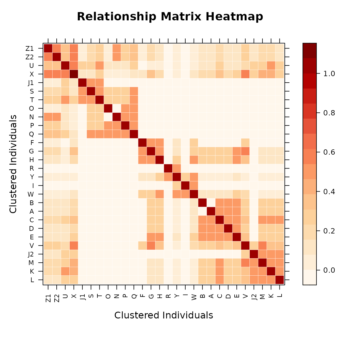

Compact Matrix — Direct Visualization

A compact pedmat object can be passed directly to vismat(). It is automatically expanded to full dimensions before rendering.

# Compact matrix: expanded automatically (message printed)
vismat(mat_compact,labelcex=0.5)
#> Expanding compact matrix (27 -> 28 individuals) for visualization.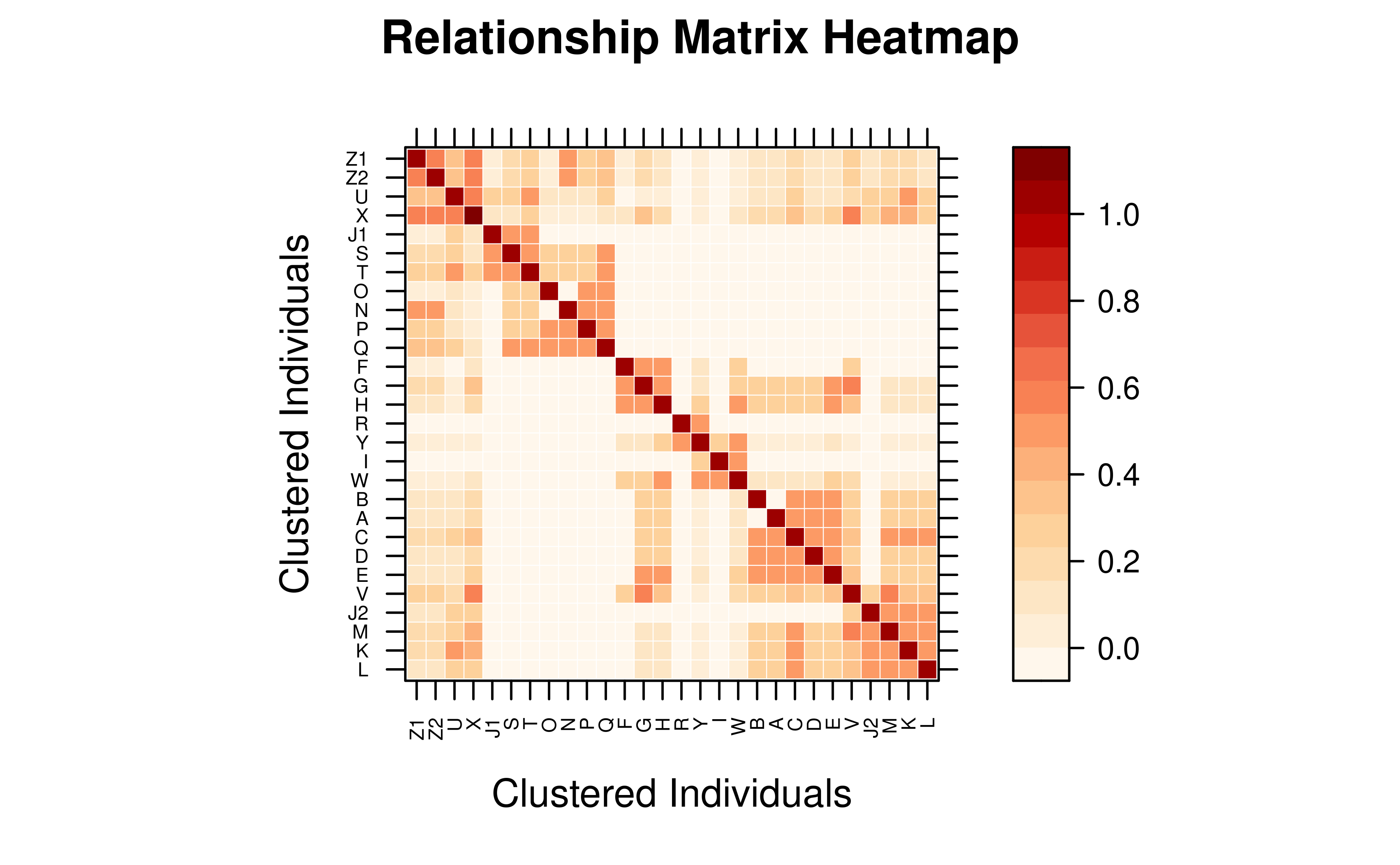

Preserve Pedigree Order

Set reorder = FALSE to keep the original pedigree order instead of re-sorting by clustering.

vismat(mat_A, reorder = FALSE, labelcex = 0.5)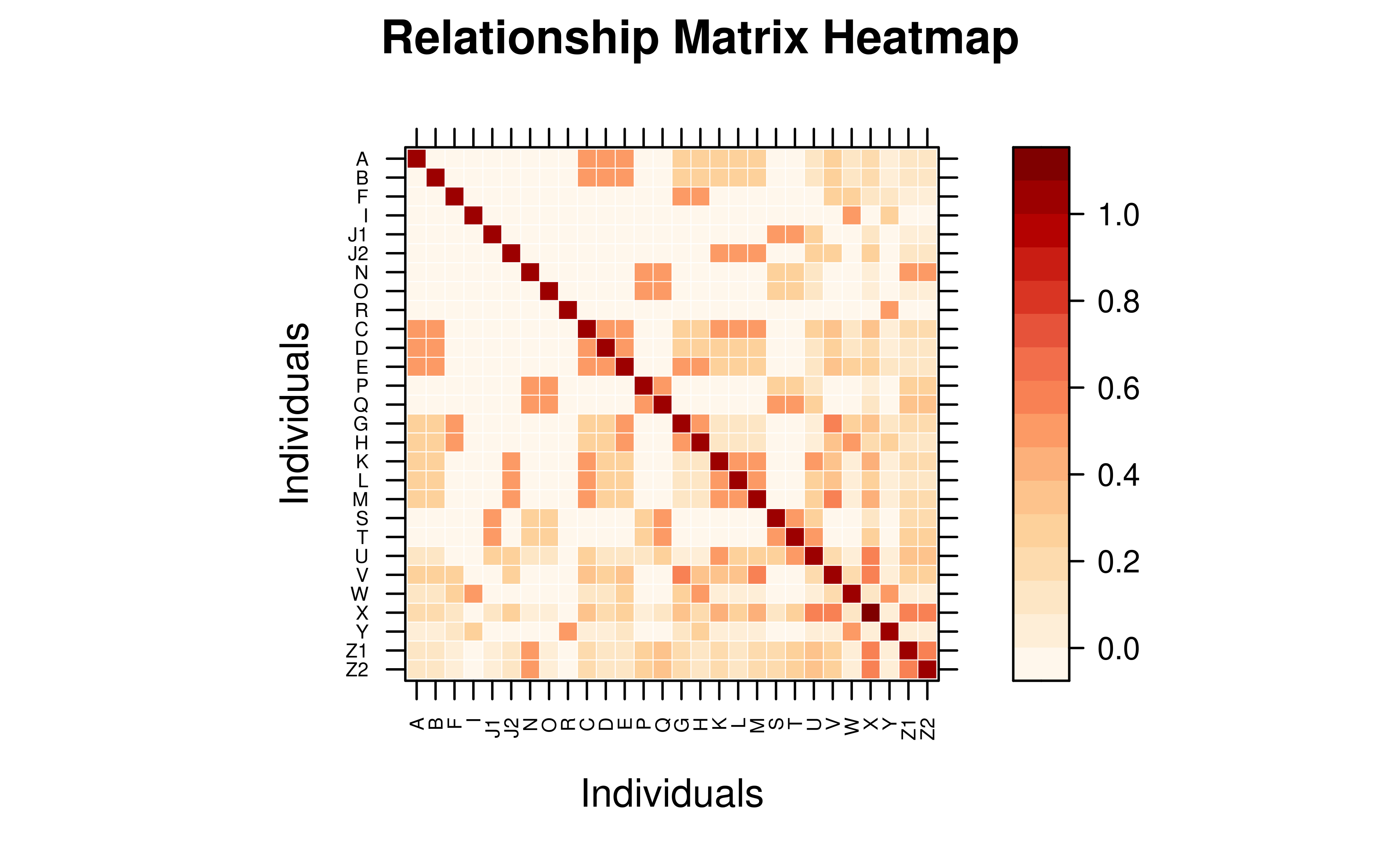

Display a Subset of Individuals

Use ids to focus on specific individuals.

target_ids <- rownames(as.matrix(mat_A))[1:8]
vismat(mat_A, ids = target_ids,
       main = "Relationship Heatmap — First 8 Individuals")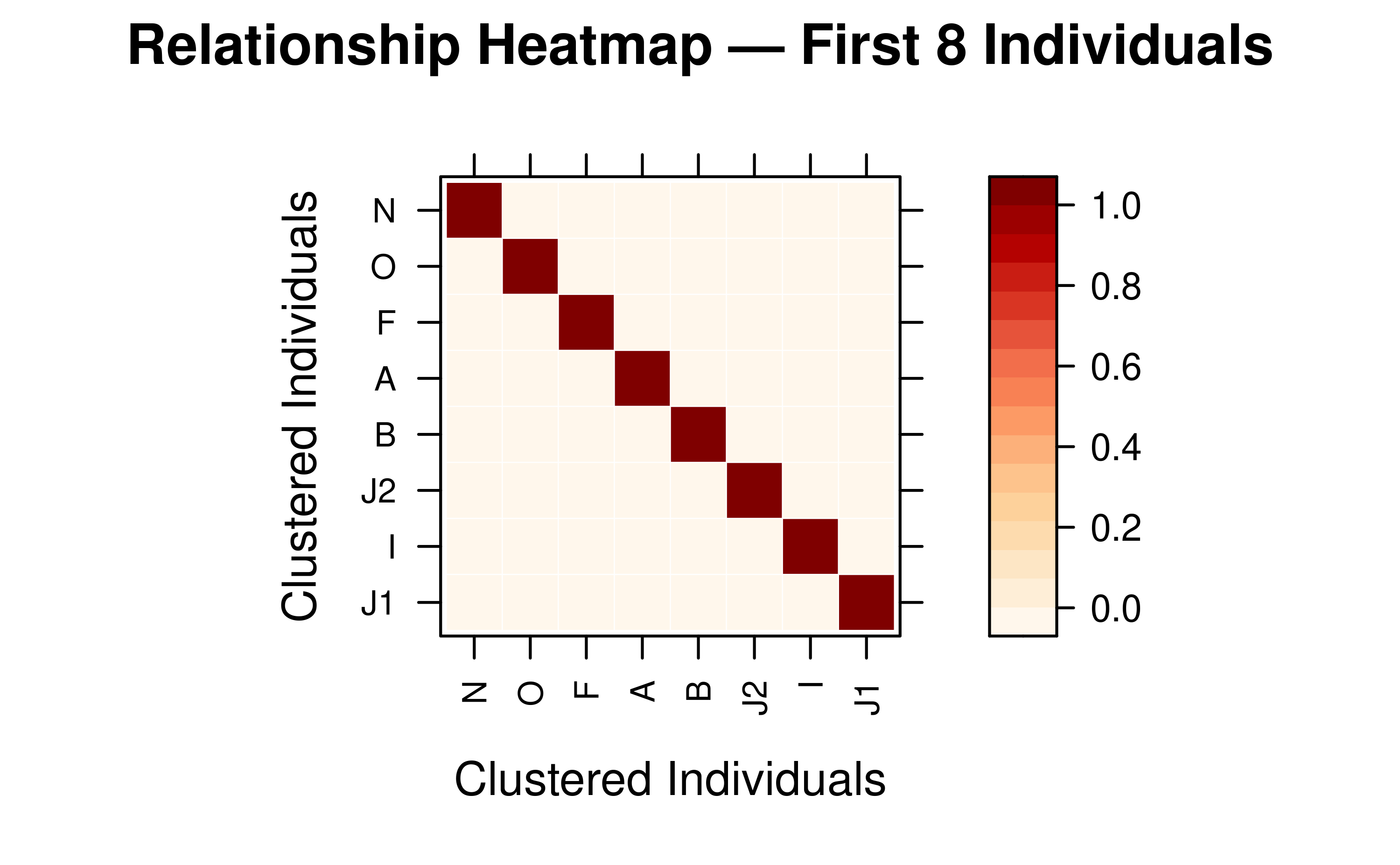

Grouping by Pedigree Column

For large populations, aggregate relationships to a group-level view using the by parameter. The matrix is reduced to mean coefficients between groups.

# Mean relationship between generations
vismat(mat_A, ped = tped, by = "Gen",
       main = "Mean Relationship Between Generations")
#> Aggregating 28 individuals into 6 groups based on 'Gen'...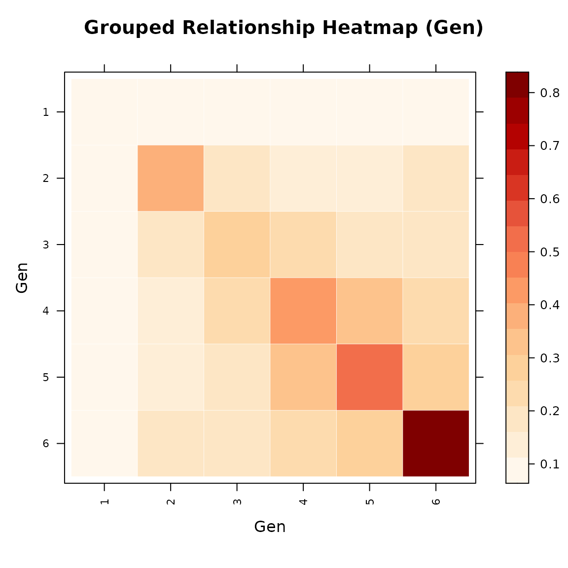

# Mean relationship between full-sib families
# (founders without a family assignment are excluded automatically)
vismat(mat_A, ped = tped, by = "Family",
       main = "Mean Relationship Between Full-Sib Families")
#> Note: Excluding 9 founder(s) with no family assignment: J1, O, N, F, R (and 4 more)
#> Aggregating 19 individuals into 11 groups based on 'Family'...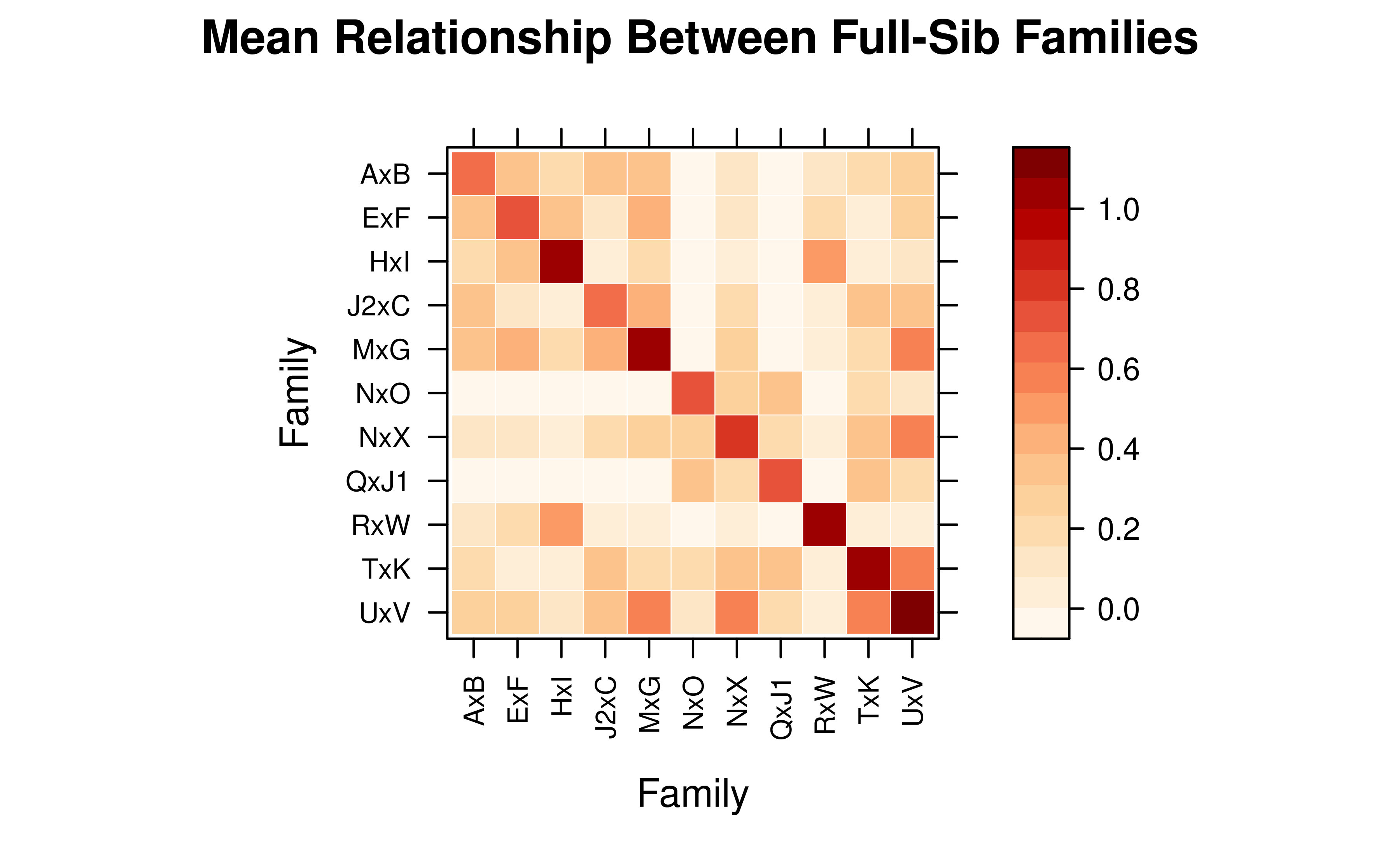

5.2 Inbreeding and Kinship Histograms

The “histogram” type displays the distribution of relationship coefficients (lower triangle) or inbreeding coefficients.

# Distribution of relationship coefficients
vismat(mat_A, type = "histogram")

6. Performance Considerations

Calculation and visualization of large matrices can be resource-intensive. vismat() applies the following automatic optimizations:

Condition	Behavior
Compact + `by`	Group means are computed directly from the compact matrix (no full expansion)
Compact, no `by`, N > 5 000	Uses compact representative view (labels show `ID (×n)`)
Compact, no `by`, N ≤ 5 000	Matrix is automatically expanded via `expand_pedmat()`
N > 2 000	Hierarchical clustering (reorder) is automatically skipped
N > 500	Individual labels are automatically hidden
N > 100	Grid lines are automatically hidden

When a compact pedmat is used with by, vismat() computes the group-level mean relationship matrix algebraically from the K×K compact matrix, including a sibling off-diagonal correction. This avoids expanding to the full N×N matrix, making family-level or generation-level visualization feasible even for pedigrees with hundreds of thousands of individuals.

The example below uses big_family_size_ped (178 431 individuals, compact to 2 626) and displays the mean additive relationship among all full-sib families in the latest generation — a computation that would be infeasible with full expansion.

data(big_family_size_ped)

tp_big <- tidyped(big_family_size_ped)
last_gen <- max(tp_big$Gen, na.rm = TRUE)

# Compute the compact A matrix for the entire pedigree
mat_big_compact <- pedmat(tp_big, method = "A", compact = TRUE)

# Focus on all individuals in the last generation that belong to a family
ids_last_gen <- tp_big[Gen == last_gen & !is.na(Family), Ind]

# vismat() aggregates directly from the compact matrix — no expansion needed
vismat(
       mat_big_compact,
       ped = tp_big,
       ids = ids_last_gen,
       by = "Family",
       labelcex = 0.3,
       main = paste("Mean Relationship Between All Families in Generation", last_gen)
)
#> Aggregating 37009 individuals into 106 groups based on 'Family'...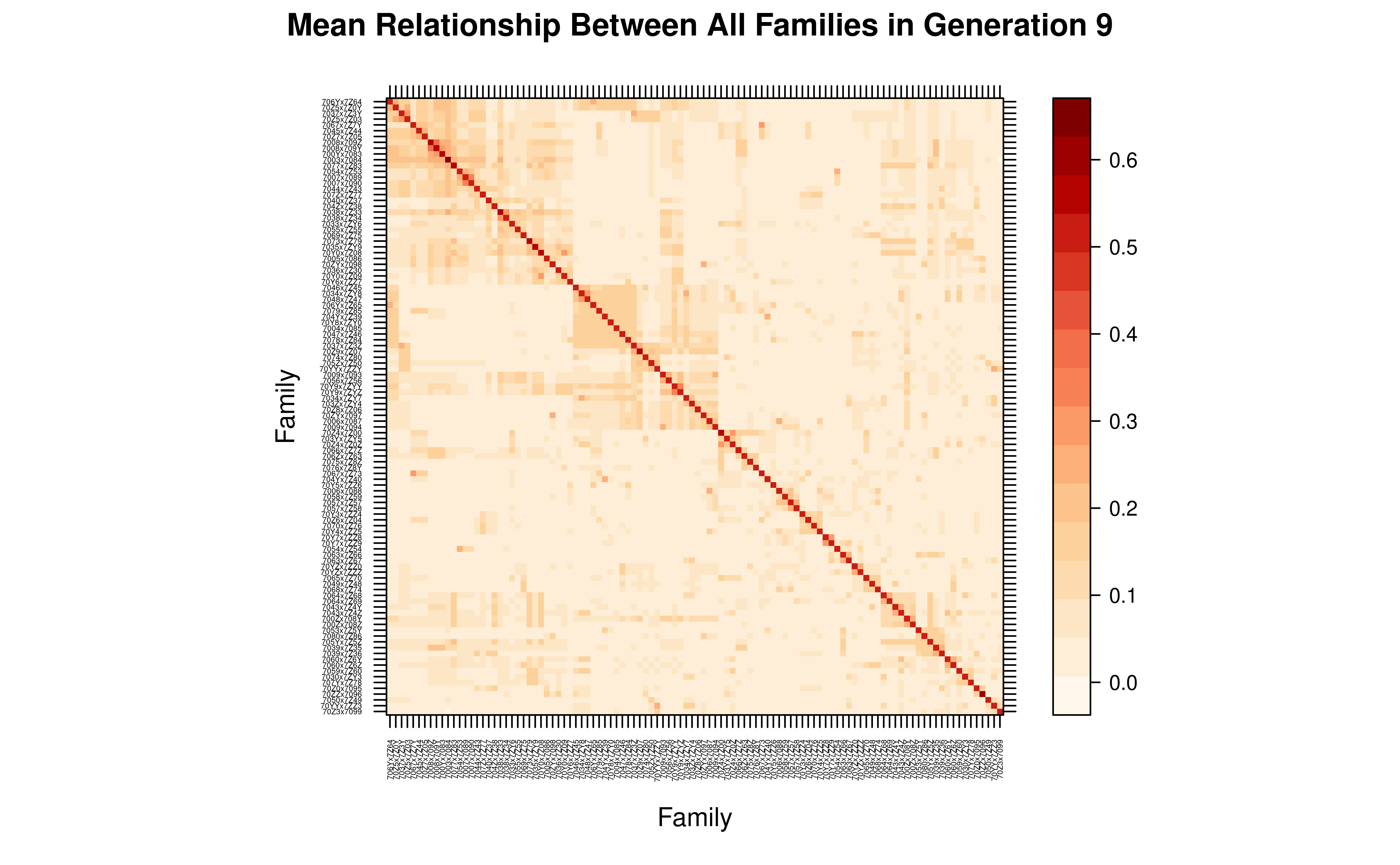

This family-level view reveals the genetic structure among all 106 families comprising 37009 individuals, computed in seconds from the compact matrix.

References

Colleau, J. J. (2002). An indirect approach to the extensive calculation of relationship coefficients. Genetics Selection Evolution, 34, 409-421.
Henderson, C. R. (1976). A simple method for computing the inverse of a numerator relationship matrix used in prediction of breeding values. Biometrics, 32(1), 69-83.
Meuwissen, T. H. E., & Luo, Z. (1992). Computing inbreeding coefficients in large populations. Genetics Selection Evolution, 24, 305-313.
Sargolzaei, M., Iwaisaki, H., & Colleau, J.-J. (2005). A fast algorithm for computing inbreeding coefficients in large populations. Journal of Animal Breeding and Genetics, 122, 325-331.

Sheng Luan

2026-07-14

1. Calculating Relationship Matrices with `pedmat()`

1.1 Supported Methods

1.2 Basic Usage

1.3 Sparse Matrix Representation

2. Matrix-Free Products with `pedprod()`

2.1 When to Use `pedprod` vs `pedmat`

2.2 Basic Usage — $A x$ (vector)

2.3 Products with $A^{-1}$

2.4 Multiple Contribution Schemes — $A X$

2.5 Practical Use Cases

Optimal Contribution Selection (OCS)

Mixed Model Equations

Founder Contribution Analysis

2.6 Performance and Scalability

3. Inspecting the Matrix

3.1 Summary Statistics

3.2 Querying Specific Relationships

4. Compact Mode for Large Pedigrees

4.1 Using `compact = TRUE`

4.2 Expanding and Querying Compacted Matrices

4.3 When to Use Compact Mode

5. Visualizing Relationship Matrices with `vismat()`

5.1 Relationship Heatmaps

Compact Matrix — Direct Visualization

Preserve Pedigree Order

Display a Subset of Individuals

Grouping by Pedigree Column

5.2 Inbreeding and Kinship Histograms

6. Performance Considerations

References

5. Calculation and visualization of relationship matrix

Sheng Luan

2026-07-14

1. Calculating Relationship Matrices with pedmat()

1.1 Supported Methods

1.2 Basic Usage

1.3 Sparse Matrix Representation

2. Matrix-Free Products with pedprod()

2.1 When to Use pedprod vs pedmat

2.2 Basic Usage — AxA x (vector)

2.3 Products with A−1A^{-1}

2.4 Multiple Contribution Schemes — AXA X

2.5 Practical Use Cases

Optimal Contribution Selection (OCS)

Mixed Model Equations

Founder Contribution Analysis

2.6 Performance and Scalability

3. Inspecting the Matrix

3.1 Summary Statistics

3.2 Querying Specific Relationships

4. Compact Mode for Large Pedigrees

4.1 Using compact = TRUE

4.2 Expanding and Querying Compacted Matrices

4.3 When to Use Compact Mode

5. Visualizing Relationship Matrices with vismat()

5.1 Relationship Heatmaps

Compact Matrix — Direct Visualization

Preserve Pedigree Order

Display a Subset of Individuals

Grouping by Pedigree Column

5.2 Inbreeding and Kinship Histograms

6. Performance Considerations

References

1. Calculating Relationship Matrices with `pedmat()`

2. Matrix-Free Products with `pedprod()`

2.1 When to Use `pedprod` vs `pedmat`

2.2 Basic Usage — $A x$ (vector)

2.3 Products with $A^{-1}$

2.4 Multiple Contribution Schemes — $A X$

4.1 Using `compact = TRUE`

5. Visualizing Relationship Matrices with `vismat()`